Decision Model

The following shows how to build and solve optimization problems in GeneDrive.jl. Decision models allow us to determine the best (optimal) strategy for achieving a goal (objective), taking into account the limitations (constraints) of our system of interest.

To set up the decision model, it is necessary to define an additional component for our data model: our problem's operational limitations (constraints). Operational constraints enter the simulation as fields of the ReleaseStrategy struct and are defined per node. View struct fields by running:

julia> ? ReleaseStrategy

Biological constraints are pre-defined within the decision model. For brevity, we will specify our example operational constraints on top of the node3 data model created previously.

# Define constraints using desired fields (re-use `release_genotype`)
node3_strategy = ReleaseStrategy(release_this_gene_index = release_genotype,
    release_this_life_stage = Male, release_start_time = 7,
    release_size_max_per_timestep = 1000)

# Assign constraints to dict of nodes
mystrategy = Dict(1 => node3_strategy)

# Build the optimization problem (re-use `node3`, `tspan`)
prob = create_decision_model(node3, tspan; node_strategy = mystrategy);

A JuMP Model
Feasibility problem with:
Variables: 16790
`JuMP.AffExpr`-in-`MathOptInterface.EqualTo{Float64}`: 5475 constraints
`JuMP.AffExpr`-in-`MathOptInterface.GreaterThan{Float64}`: 1095 constraints
`JuMP.AffExpr`-in-`MathOptInterface.LessThan{Float64}`: 2191 constraints
`JuMP.QuadExpr`-in-`MathOptInterface.EqualTo{Float64}`: 3285 constraints
`JuMP.VariableRef`-in-`MathOptInterface.EqualTo{Float64}`: 3291 constraints
`JuMP.VariableRef`-in-`MathOptInterface.GreaterThan{Float64}`: 13499 constraints
`JuMP.VariableRef`-in-`MathOptInterface.LessThan{Float64}`: 359 constraints
Nonlinear: 3285 constraints
Model mode: AUTOMATIC
CachingOptimizer state: EMPTY_OPTIMIZER
Solver name: Ipopt
Names registered in the model: E, E_con_A0, E_con_A1, E_con_B0, E_con_B1, F, F_con_0, F_con_1, L, L_con_A0, L_con_A1, L_con_B0, L_con_B1, M, M_con_0, M_con_1, P, P_con_A0, P_con_A1, P_con_B0, P_con_B1, Sets, control_F, control_M, control_equivalence, control_limit_schedule_lower_F, control_limit_schedule_lower_M, control_limit_schedule_upper_F, control_limit_schedule_upper_M, control_limit_total_F, control_limit_total_M, mate_bound, migration_E, migration_L, migration_M, migration_P, release_location

To solve the decision model as an optimization, a goal (objective) must be supplied. However, even in the absence of an objective function we can derive useful information: without an objective, the solution method auto-selected by GeneDrive.jl acts as a nonlinear solver and allows us to compare the behavior of our dynamic and decision models.

# Solve
sol = solve_decision_model(prob);

# Format all results for analysis
results = format_decision_model_results(sol);

Dict{Any, Any} with 8 entries:
  :node_1_scenario_1_organism_1_P => 365×3 DataFrame…
  :node_1_scenario_1_organism_1_E => 365×3 DataFrame…
  :node_1_scenario_1_organism_1_F => 365×3 DataFrame…
  :node_1_scenario_1_organism_1_M => 365×3 DataFrame…
  :node_1_scenario_1_organism_1_L => 365×3 DataFrame…
  :node_1_organism_1_control_M    => 365×3 DataFrame…
  :Time                           => [1, 2, 3, 4, 5, 6, 7, 8, 9, 10  …  356, 35…
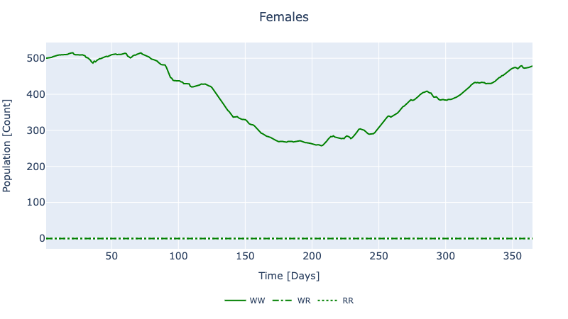
  :node_1_organism_1_control_F    => 365×3 DataFrame…

To visualize a subset of the results, run plot_decision_ridl_females(sol). Because no objective function was specified, this output should qualitatively match those from the dynamic model when no intervention is conducted (i.e. when using the same data model, and no RIDL release object is passed to solve_dynamic_model).